Double Pendulum MATLAB Files

Double Pendulum

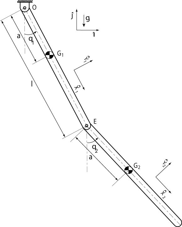
    To illustrate the basics of dynamic MATLAB simulations, we will look at the simulation of a double pendulum. This example will cover derivation of equations of motion by hand, symbolic derivation of the equations of motion in MATLAB, simulation of the equations of motion, and simulation checks. Figure 1 depicts the double pendulum with the assumed coordinate systems, dimensions and angles.

Figure 1. Double Pendulum with Assumed Coordinate Systems, Dimensions and Angles

Finding the Equations of Motion

    To find the equations of motion for a dynamic system, we use the Newton-Euler method. This method involves balancing the linear and angular momentum of a system. For our example, we will only perform angular momentum balances. Angular momentum balances must take place about a point and can be expressed as,

    That is the sum of the moments is equal to the rate of change of angular momentum.

    To find the equations of motion for the double pendulum, we will perform two angular momentum balances, one at point O and one at point E. Figure 2 depicts the free body diagrams for the two angular momentum balances.

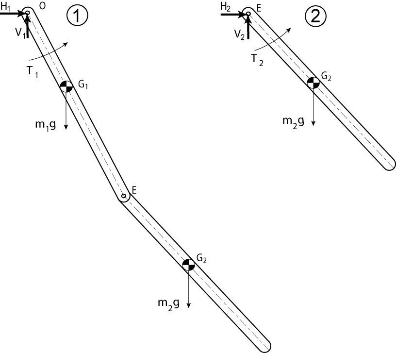
Figure 2. Free Body Diagrams of a) Both link attached, Angular Momentum balance about point O gives one equation b) Second link only, Angular Momentum balance about point E gives the second equation of motion

    From the two free body diagrams, we get,

    where,

                                                                                                                    Masses of links 1 and 2

                                                                                                                        Inertia of links 1 and 2

                                                                                                                            Gravitational acceleration

                                                                                                                      Angular accelerations of links 1 and 2

                                                                                                                  Accelerations of links 1 and 2

                                                                                                                      External torques on links 1 and 2

                                                                                                                        External moment about point A

                                                                                                                        Rate of change of angular momentum about point A

                                                                                                                        Position vector from point B to A

                                                                                                                         Unit vectors along x, y and z axes

    The equations of motion result from setting and .

Symbolic Deviation of the Equations of Motion in MATLAB

    The derivation of the equations of motion for a given system can be done symbolically in MATLAB to reduce the number of errors a typical hand written solution can produce and to arrange the equations in such a way as to use them in a numerical MATLAB simulation. The full derivation code can be found at the end of this section,

    We must first determine the symbolic variables that will be required to solve the problem. Any variable such angles or distances and its derivatives should be defined as symbolic. Additionally, any parameter in the problem such as length or radius should also be symbolic. This allows us to have as general solution as possible.

syms a l m1 m2 I1 I2 g T1 T2

syms q1 q2 u1 u2 ud1 ud2

    We then define the coordinate frames we set up in the solution to our problem and any position vectors that will be needed for plotting and/or solving the problem.

%%%%%%% Reference frames %%%%%%%

i = [1 0 0]; j = [0 1 0]; k = [0 0 1];

X1 = sin(q1)*i - cos(q1)*j; Y1 = cos(q1)*i + sin(q1)*j;

X2 = sin(q2)*i - cos(q2)*j; Y2 = cos(q2)*i + sin(q2)*j;

%%%%%%% Position vectors %%%%%%

r_O_G1 = a*X1;

r_O_E = l*X1;

r_E_G2 = a*X2;

r_O_G2 = r_O_E + r_E_G2;

    We now define the angular velocities, angular accelerations, mass velocities and mass accelerations in terms of the symbolic variables and position vectors.

%%%%%% Angular velocities and accelerations %%%%%

om1 = u1*k; om2 = u2*k;

al1 = ud1*k; al2 = ud2*k;

%%%%% Velocties (not needed here) and acelerations of masses %%%%

v_O = 0;

v_G1 = v_O + cross(om1,r_O_G1);

v_E = v_O + cross(om1,r_O_E);

v_G2 = v_E + cross(om2,r_E_G2);

a_O = 0;

a_G1 = a_O + cross(om1,cross(om1,r_O_G1)) + cross(al1,r_O_G1);

a_E = a_O + cross(om1,cross(om1,r_O_E)) + cross(al1,r_O_E);

a_G2 = a_E + cross(om2,cross(om2,r_E_G2)) + cross(al2,r_E_G2);

    Next, we code the statements for the angular momentum balance. Each angular momentum balance will result in one equation of motion. Since this is a planar problem, the equations of motion will be in the direction of resulting vector.

%%%%% Angular Momentum %%%%%%%%%%%%%%%%%%%%%%

M_O = cross(r_O_G1,-m1*g*j) + cross(r_O_G2,-m2*g*j) + T1*k;

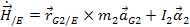
Hdot_O = cross(r_O_G1,m1*a_G1) + I1*al1 + cross(r_O_G2,m2*a_G2) + I2*al2;

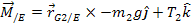
M_E = cross(r_E_G2, -m2*g*j) + T2*k;

Hdot_E = cross(r_E_G2, m2*a_G2) + I2*al2;

%%%%% Equations of motion %%%%%%%%%%%%%%%%%%

AMB_O = M_O - Hdot_O;

AMB_E = M_E - Hdot_E;

%%% The k component has the equations of motion %%%

eqn1 = AMB_O(3);

eqn2 = AMB_E(3);motion result from setting and .

eqn1 = eqn1 - eqn2; %%There is no need to do this but we do it to make the resulting M matrix symmetric

    We now want to manipulate the equations to fit the form of,

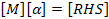
    where

    We can get by plugging in zero for both angular accelerations in each of the equations of motion and taking the negative of the result. The negation is required because we need to move those terms to the other side. Now, we can get the first column of by substituting one for and zero for in each angular momentum balance and adding to remove any constants. To get the second column of , we perform the same operations with and .

RHS1 = -subs(eqn1,[ud1 ud2],[0 0]) %negative sign because we want to take RHS to the right eventually

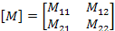
M11 = subs(eqn1,[ud1 ud2],[1 0]) + RHS1

M12 = subs(eqn1,[ud1 ud2],[0 1]) + RHS1

RHS2 = -subs(eqn2,[ud1 ud2],[0 0])

M21 = subs(eqn2,[ud1 ud2],[1 0]) + RHS2

M22 = subs(eqn2,[ud1 ud2],[0 1]) + RHS2

%%%%%%% Final system [M] [alpha] = [RHS] %%%%%%%%%%%%%%%

M = [M11 M12; M21 M22];

RHS = [RHS1; RHS2];

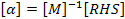
    When we solve for the angular accelerations, we will multiply the inverse of the mass matrix with . We will not symbolically invert the mass matrix since doing so is computationally expensive compared to inverting it numerically.

    We now have the necessary matrices to simulate the double pendulum. In this simpler case, we can copy and paste the equations of motion in the simulation m-file. In more complicated problem with more degrees of freedom, the resulting matrices are much larger and it is easier to have MATLAB create a m-file that is already setup for simulation. This case will be demonstrated in the next section.

    In addition to deriving the equations of motion, we can also derive the kinetic and potential energy equations. This is a simple task of converting the equations into the symbolic variables already defined in the file.

%%%% Total energy (as a check on equations) %%%%

KE = simple(0.5*m1*(v_G1(1)*v_G1(1)+v_G1(2)*v_G1(2)) + 0.5*m2*(v_G2(1)*v_G2(1)+v_G2(2)*v_G2(2)) + 0.5*I1*u1*u1 + 0.5*I2*u2*u2)

PE = -m1*g*a*cos(q1) - m2*g*(l*cos(q1) + a*cos(q2))

Creating a Simulation in MATLAB

    Now that we have the equations of motion, we can set up a simulation. The simulation will be setup into 3 parts: the driver which will integrate the equations of motion and create an animation, the right hand side of the equations of motion, and the energy equations.

    First, we need to set up a file for the equations of motion. The m-file will contain a single function that takes in a time, set of angles and their derivatives, and parameters and returns the first and second derivatives of the angles. In this file, we need to put the M and RHS matrices and plug in the parameters, angles and derivatives. We can then find the angular accelerations by,

    Additionally, we need to set up a m-file for the energy. Similarly to the equation of motion file, this file takes in the time, positions and derivatives, and parameters and returns the kinetic and potential energy at that particular instance.

    We can now create the driver for the simulation. First, we must define the parameters, initial conditions, and a vector of times to integrate over.

%%%%%%%%% INITIALIZE PARAMETERS %%%%%%

%Mechanical parameters.

m1 = 1; m2 = 1; % masses

I1 = 0.5; I2 = 0.5; % inertias about cms

l = 1; % length of links

a = .5; % dist. from O to G1 and E to G2 (see figures)

g = 10;

% Initial conditions and other settings.

framespersec=50; %if view is not speeded or slowed in dbpend_animate

T=10; %duration of animation in seconds

tspan=linspace(0,T,T*framespersec);

q1 = pi/2-0.1; %angle made by link1 with vertical

u1 = 0; %abslolute velocity of link1

q2 = pi ; %angle made by link2 with vertical

u2 = 0; %abslolute velocity of link2

z0=[q1 u1 q2 u2]';

    We then must set the absolute and relative error tolerances for the integration.

options=odeset('abstol',1e-9,'reltol',1e-9);

    We can now choose an ode function. There are three we can choose from ode45, ode113, and ode23. We will choose ode113 because it is relatively faster than the others at higher precisions. Using ode113 and inputting the time span, initial conditions and parameters, we can integrate the equations of motion over the time period allotted.

%%%%%%% INTEGRATOR or ODE SOLVER %%%%%%%

[t z] = ode113('dbpend_rhs',tspan,z0,options, ...

m1, m2, I1, I2, l, a, g);

    Ode113 will return the same time period and the resulting angles and angular velocities. Post processing can now be done. First, we create an animation. This is done by repeatedly plotting the positions of the masses in the same plot over the specified time span.

figure(1)

for i=1:length(tspan)

pause(.01)

xm1=-l*sin(z(i,1));

ym1=-l*cos(z(i,1));

xm2=xm1-l*sin(z(i,3));

ym2=ym1-l*cos(z(i,3));

plot([0],[0],'ko','MarkerSize',3); %pivot point

hold on

plot([0 xm1],[0 ym1],'r','LineWidth',2);% first pendulum

plot([xm1 xm2],[ym1 ym2],'b','LineWidth',2);% second pendulum

axis([-2*l 2*l -2*l 2*l]);

axis square

hold off

end

    Additionally, we can plot the time histories of the angles and velocities.

figure(2)

plot(t,z(:,1),t,z(:,3));

xlabel('time (s)'); ylabel('position (rad)');

Checking the Simulation

    After integrating the equations of motion in MATLAB and creating an animation, we need to ensure that the simulation is correct. One way to do this is to ensure that energy is conserved. In our derivation of the equations of motion of the double pendulum, we also derived the kinetic energy and potential energy of the system. The total energy of the system, the kinetic energy plus the potential energy, must be conserved. Since the total energy is a function of the state variables and their derivatives, which is what our integration produced, we can calculate the total energy for each time step and plot the difference between each step.

for i=1:length(t)

[KE(i), PE(i)] = dbpend_energy(t(i),z(i,:),m1, m2, I1, I2, l, a, g);

end

TE = KE + PE;

TE_diff = diff(TE);

figure(3)

plot(t(1:end-1),TE_diff)

    The resulting plot should be very close to zero with some spikes that are less than the tolerance of the integrator.

    Another way of checking a simulation is to reduce the problem to a simpler problem which can be solved by hand. In the case of the double pendulum, we can reduce the problem to a single pendulum with a point mass at the end and a massless rod. We can do this in the simulation by setting the parameters to the following values:

    The second pendulum will still be present in the animation but will not move.

Figure 3. Single Pendulum showing assumed coordinate axis, distance, and angles

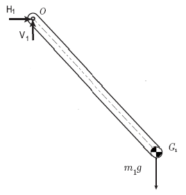
Figure 4. FBD of the single pendulum

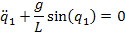
    From Figure 4, we can perform an angular momentum balance about point O.

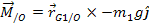
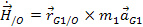
    The result of this balance is the differential equation,

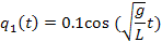
    Linearizing this equation about and and using the initial conditions, we can find a closed form of the solution by hand.

    We can compare the simulation's result with our analytic result by adding the following lines to the end of our code for the driver,

figure(4)

plot(t,z(:,1),t,.1*cos(sqrt(g*t/l));

xlabel('time (s)'); ylabel('position (rad)');

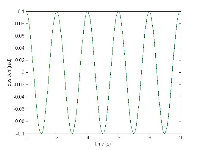
Figure 5. Plot of the Reduced Single Pendulum Model and Hand Derivate Equation of Motion

From the above result, we can see that the simulation and analytic result match very closely. Between this result and the conservation of energy, we have shown that the simulation is valid. There are several other ways of reducing the double pendulum. If we set , we will get the same result as above. Another way is to set .Additionally, we can lock the angle . This will result in a single pendulum of length .

Double Pendulum MATLAB Files